0%

There are two ways to calculate the attention in transformer: one is $\text{Attention(Q, K, V)}=\text{softmax}(\frac{QK^T}{\sqrt{d_k}})\times V$ same as in Attention Is All You Need, the other is $\text{Attention(Q, K, V)}=V \times\text{softmax}(\frac{K^TQ}{\sqrt{d_k}})$ from here. Depending on different context, both are correct. The key point is How You Organize the Input.

I manage to go over the vector version of the attention and then derive the matrix form.
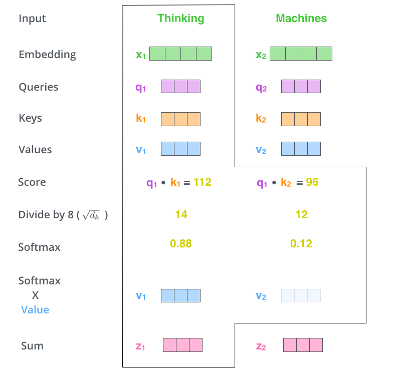
Vector Version

The aim of the attention mechanism is to map a query and a set of key-value pairs to an output.

Suppose we have sets of vectors: input $x$, query, key, and value with dimensions $d_p$, $d_q$, $d_k$, and $d_v$ respectively, where $d_q = d_k$ For each input $x_i$, there are corresponding $q_i$, $k_i$, and $v_i$.

Denote

$$
a_{1, i} = \frac{q_1 \cdot k_i}{\sqrt{d_k}} \text{, where }i=1, 2, \dots
$$

What $a_{1, i}$ means is a vector of products between the input $x_1$ and other keys. The name, scaled dot-product, is from dividing $\sqrt{d_k}$. It’s introduced to tackle the problem made by magnitude in computation, and also can be checked in the article.

Then, the output 1 is

$$
\begin{align*}
o_1 &= \sum_i \hat{a_{1, i}} \cdot v_i &\text{where } \hat{a_{1, i}} = \text{softmax}(a_{1, i}), i=1, 2, \dots
\end{align*}
$$

The softmax function converts a vector of numbers into a vector of probabilities [wiki], and the outcome 1 is the sum of the scalar multiplications of the scalar $\hat{a_1, i}$ and the vector $v_i$.

Usually, the result of the attention function has the same shape of the input.

an example for reference

Matrix Version

Different from the vector version, there is one more step before the attention calculation for the matrix version. The query, key and value are not given directly, but they are computed from matrices $W^Q$, $W^k$, and $W^v$.

Suppose we have the input with shape $[n, p]$. The weight matrices are going to be $[p, d_q]$, $[p, d_k]$, and $[p, d_v]$. $n$ is just the number of inputs, or in another words, the batch size.

Then,

$$
Q: [n, d_q]
$$
$$ K: [n, d_k]
$$

$$ V: [n, d_v]
$$

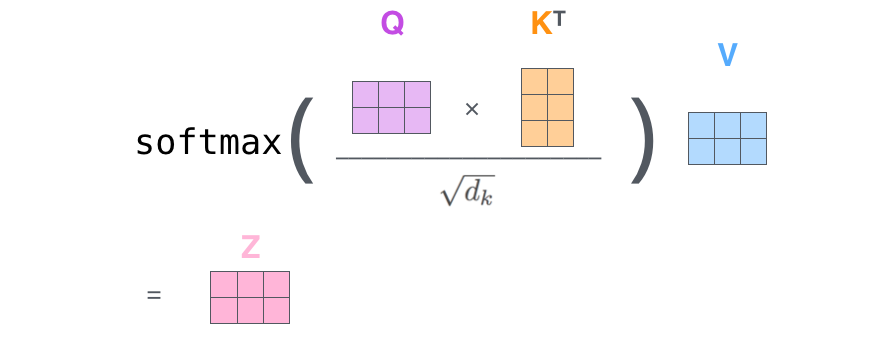
Since each row of Q has to multiply each row in K, we can transpose the K and make a matrix multiplication $Q \cdot K^T$. The result is a $n \times n$ matrix, each row is the result corresponding to the vector version. For example, in the first row there are elements $a_{1, 1}, a_{1, 2}, \dots, a_{1, i},$.

$$
\begin{pmatrix}
\alpha_{1, 1}=q^1\cdot k^1 & \alpha_{1, 2}=q^1\cdot k^2 & \cdots & \alpha_{1, i}=q^1\cdot k^k \\
\vdots & \alpha_{2,2} & \cdots & \vdots \\
\alpha_{n, 1} & \cdots & \cdots & \alpha_{n,i}
\end{pmatrix}
$$

Dividing $\sqrt{d_k}$ and applying softmax function do not change the shape of this $n \times n$ matrix, so we are going to multiply V with a $n \times n$ matrix.

Please pay attention (pun),

$$
\begin{align*}
o_1 &=\sum_{i}\hat{a}_{1,i}v_i \\
&= \hat{a}_{1,1}v_1 + \hat{a}_{1,2}v_2 + \cdots + \hat{a}_{1,i}v_i \\
&= \begin{pmatrix}
v_1 & v_2 & \dots & v_i
\end{pmatrix} \begin{pmatrix}
\hat{a}_{1,1} \\
\hat{a}_{1,2} \\
\vdots \\
\hat{a}_{1,i}
\end{pmatrix} \\
&= \begin{pmatrix}
\hat{a}_{1,1} & \hat{a}_{1,2} & \cdots & \hat{a}_{1,i}
\end{pmatrix}\begin{pmatrix}
v1 \\ v2 \\ \vdots \\ v_i
\end{pmatrix}
\end{align*}
$$

any $\hat{a}$ is a scalar, but any v is a vector.

Therefore, we can have

$$
\begin{align*}
\text{Attention(Q, K, V)}&=\text{softmax}(\frac{QK^T}{\sqrt{d_k}})\times V\\
&=\text{softmax}(\frac{QK^T}{\sqrt{d_k}})\times \begin{pmatrix}
v1 \\ v2 \\ \vdots \\ v_i
\end{pmatrix}.
\end{align*}
$$

This is exactly what this figure is doing(Adding a mask is optional).

scaled dot-product attention

Jay’s figures perfectly express shapes of matrices in calculation.
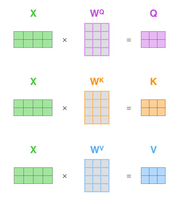
computing Q, V, K
computing attention

the other Formula

However, the matrix multiplication isn’t invertable like scalar multipication. The formula above cannot give the anticipant results, if we cancate vectors of inputs colomn by column into a matrix. In this situation, we have to also transpose the Q, K, V matrices and use the second formula.

$$
\text{Attention(Q, K, V)}=V \times\text{softmax}(\frac{K^TQ}{\sqrt{d_k}})
$$

Conclusion

Understanding the vector version can help to choose the right formula. Most of the case, we use $\text{Attention(Q, K, V)}=\text{softmax}(\frac{QK^T}{\sqrt{d_k}})\times V$, such as in PyTorch. But be careful, if the input is a $[p, n]$ matrix.

Code

1
2
3
4
5
6
7
8
9
10
11
12
13
14
15
16
17
18
19
20
21
22
23
24
25
26
27
28
29
30
31
32
33
34
35
36
37
38
39
def compute_QKV(embedding: torch.Tensor,
Wq: torch.Tensor,
Wk: torch.Tensor,
Wv: torch.Tensor) -> typing.Tuple:
"""
compute Q, V, K matrices by embedding and weights
:param embedding: shape [n, p]
:param Wq: shape [p, d_k]
:param Wv: shape [p, d_v]
:param Wk: shape [p, d_k]
:return: Tuple[Q, V, K]
where Q: shape [n, d_k]
where K: shape [n, d_k]
where V: shape [n, d_v]
"""
return torch.matmul(embedding, Wq), torch.matmul(embedding, Wk), torch.matmul(embedding, Wv)

def scaled_dot_product(Q: torch.Tensor,
K: torch.Tensor) -> torch.Tensor:
"""

:param Q: shape [n, d_k]
:param K: shape [n, d_k]
:return: Tensor shape [n, n]
"""
dk = K.shape[1]
return torch.matmul(Q, K.T) / torch.sqrt(torch.tensor(dk))

def attention(A: torch.Tensor,
V: torch.Tensor) -> torch.Tensor:
"""

:param A: shape [n, n]
:param V: shape [n, d_v]
:return: Tensor with shape [n, d_v]
"""
A_prime = torch.softmax(A, dim=1)
assert 0.9 < A_prime[0].sum() < 1.1 # do softmax row by row
return torch.matmul(A_prime, V)

Example

Done by the first approach

$$
\text{Attention(Q, K, V)}=\text{softmax}(\frac{QK^T}{\sqrt{d_k}})\times V
$$

1
2
3
4
5
6
7
8
9
10
11
12
13
14
15
16
17
18
19
20
21
22
23
24
embeddings = torch.tensor([
[1, 1, 1, 0],
[1, 2, 1, 0],
[0, 1, 0, 1],
[0, 1, 1, 0]
])
Wq = torch.tensor([
[1, 0, 1],
[1, 1, 1],
[0, 0, 1],
[1, 0, 0]
])
Wk = torch.tensor([
[1, 0, 0],
[1, 1, 1],
[1, 0, 1],
[0, 1, 0]
])
Wv = torch.tensor([
[1, 2, 0],
[1, 3, 1],
[1, 0, 2],
[1, 1, 0]
])
1
2
3
4
5
6
7
8
9
Q, K, V = compute_QKV(embeddings, Wq, Wk, Wv)


A = scaled_dot_product(Q, K)


Aprime = torch.softmax(A, dim=1)
torch.matmul(Aprime, V.type(torch.float))

tensor([[3.9492, 7.8588, 3.9577],
        [3.9924, 7.9784, 3.9934],
        [3.8407, 7.5669, 3.8595],
        [3.7902, 7.4482, 3.8228]])
1
attention(A.type(torch.float), V.type(torch.float))
tensor([[3.9492, 7.8588, 3.9577],
        [3.9924, 7.9784, 3.9934],
        [3.8407, 7.5669, 3.8595],
        [3.7902, 7.4482, 3.8228]])

Done by the second approach

$$
\text{Attention(Q, K, V)}=V \times\text{softmax}(\frac{K^TQ}{\sqrt{d_k}})
$$

1
2
3
4
5
6
7
8
9
10
11
12
13
14
15
16
17
18
19
20
21
22
23
24
25
26
27
28
29
30
31
32
33
34
35
36
37
38
39
def compute_QKV2(embedding: torch.Tensor,
Wq: torch.Tensor,
Wk: torch.Tensor,
Wv: torch.Tensor) -> typing.Tuple:
"""
compute Q, V, K matrices by embedding and weights
:param embedding: shape [p, n]
:param Wq: shape [d_k, p]
:param Wv: shape [d_v, p]
:param Wk: shape [d_k, p]
:return: Tuple[Q, V, K]
where Q: shape [d_k, n]
where K: shape [d_k, n]
where V: shape [d_v, n]
"""
return torch.matmul(Wq, embedding), torch.matmul(Wk, embedding), torch.matmul(Wv, embedding)

def scaled_dot_product2(Q: torch.Tensor,
K: torch.Tensor) -> torch.Tensor:
"""

:param Q: shape [d_k, n]
:param K: shape [d_k, n]
:return: Tensor shape [n, n]
"""
dk = K.shape[0]
return torch.matmul(K.T, Q) / torch.sqrt(torch.tensor(dk))

def attention2(A: torch.Tensor,
V: torch.Tensor) -> torch.Tensor:
"""

:param A: shape [n, n]
:param V: shape [d_v, n]
:return: Tensor with shape [d_v, n]
"""
A_prime = torch.softmax(A, dim=0)
assert 0.9 < A_prime[:, 0].sum() < 1.1 # do softmax column by column
return torch.matmul(V, A_prime)

Following the resoning above, if we transpose the input and weight matrices of Q, K, and V, the result should be the same.

1
2
3
4
Q2, K2, V2 = compute_QKV2(embeddings.T, Wq.T, Wk.T, Wv.T)
A2 = scaled_dot_product2(Q2, K2)
# transpose the result making it more readable
attention2(A2.type(torch.float), V2.type(torch.float)).T
tensor([[3.9492, 7.8588, 3.9577],
        [3.9924, 7.9784, 3.9934],
        [3.8407, 7.5669, 3.8595],
        [3.7902, 7.4482, 3.8228]])

This blog talks about one advantage of Optional<>. It’s nothing fancy and just warps up pieces of code into a new class. Here comes the question: why should I use it? I can do all on my own! The following two example will demonstrate how to use Optional<> to express the idea of empty value and to prevent logical flaws.


Let’s start with simpler case: the binary search. This algorithm utilizes the order of the given list and searches the index of the target. If not found, -1 will be return. So far, so good. As -1 isn’t a valide value of indices.

1
2
3
4
5
6
7
8
9
10
11
12
13
14
15
16
17
18
19
public static int bSearch(List<Integer> list, int target) {
int ret = -1;

int low = 0;
int high = list.size();
int mid = 0;

while (low <= high) {
mid = (low + high) / 2;
if (list.get(mid) == target) {
return mid;
} else if (list.get(mid) < target) {
low = mid + 1;
} else {
high = mid - 1;
}
}
return ret;
}

We can refactor the code with Optional<>. The logic here is simple. We need a variable to store the result, but it could be empty. The Optional<Integer> emphasised the target coulde not be in the list instead of putting a misleading -1.

1
2
3
4
5
6
7
8
9
10
11
12
13
14
15
16
17
18
19
public static Optional<Integer> search(List<Integer> list, int target) {
Optional<Integer> ret = Optional.empty();

int low = 0;
int high = list.size();
int mid = 0;

while (low <= high) {
mid = (low + high) / 2;
if (list.get(mid) == target) {
return Optional.of(mid);
} else if (list.get(mid) < target) {
low = mid + 1;
} else {
high = mid - 1;
}
}
return ret;
}

In short, this example shows how to take the advantage of Optional<> to express the uncertain or un-computed idea in coding.

However, this example cannot even convince me to use Optional<> anywhere. An agreement on -1 does work. Why should I use another box to do that?

Here comes the other example.

It’s a Java version solution for the set-covering problem on page 151 [1]. It tends to find the approximately letest stations covering all the states using the greedy algorithm. Everytime it goes through the map stations to find one that can cover most states in statesNeeded. Once founded, covered states will be removed from statesNeeded, and the station name will be put in finalStations. Repeat, until statesNeeded is empty.

Now, look at this code and tell whether it is robust.

1
2
3
4
5
6
7
8
9
10
11
12
13
14
15
16
17
18
19
20
21
22
23
24
25
26
27
28
29
30
public static void main(String... args) {
var statesNeeded = new HashSet<>(Arrays.asList("mt", "wa", "or", "id", "nv", "ut", "ca", "az"));
var stations = new LinkedHashMap<String, Set<String>>();

stations.put("kone", new HashSet<>(Arrays.asList("id", "nv", "ut")));
stations.put("ktwo", new HashSet<>(Arrays.asList("wa", "id", "mt")));
stations.put("kthree", new HashSet<>(Arrays.asList("or", "nv", "ca")));
stations.put("kfour", new HashSet<>(Arrays.asList("nv", "ut")));
stations.put("kfive", new HashSet<>(Arrays.asList("ca", "az")));

var finalStations = new HashSet<String>();
while (!statesNeeded.isEmpty()) {
String bestStation = null;
var statesCovered = new HashSet<String>();

for (var station : stations.entrySet()) {
var covered = new HashSet<>(statesNeeded);
covered.retainAll(station.getValue());

if (covered.size() > statesCovered.size()) {
bestStation = station.getKey();
statesCovered = covered;
}
}
statesNeeded.removeIf(statesCovered::contains);
finalStations.add(bestStation);
}
System.out.println(finalStations); // [ktwo, kone, kthree, kfive]
}

Of course not. It just works fine with this input. The weakness is String bestStation = null;. In some scenarios, finalStations.add(bestStation); adds a null. If initialize bestStation with empty String “”, the case is the same, and it just replaces the null to “”. However, the set statesNeeded works as your intention. If statesCovered is empty, saying no element is going to be remove from statesNeeded, then statesNeeded stays the same. Because empty set is an identity element of set operations.

In most of the case, we need to filter out empty strings. Like this. Different from the binary search case, this time you may forget the filter operation.

1
2
3
4
5
6
7
8
9
10
11
12
13
14
15
16
17
18
19
20
21
22
23
24
25
26
27
28
29
30
31
32
public static void main(String... args) {
var statesNeeded = new HashSet<>(Arrays.asList("mt", "wa", "or", "id", "nv", "ut", "ca", "az"));
var stations = new LinkedHashMap<String, Set<String>>();

stations.put("kone", new HashSet<>(Arrays.asList("id", "nv", "ut")));
stations.put("ktwo", new HashSet<>(Arrays.asList("wa", "id", "mt")));
stations.put("kthree", new HashSet<>(Arrays.asList("or", "nv", "ca")));
stations.put("kfour", new HashSet<>(Arrays.asList("nv", "ut")));
stations.put("kfive", new HashSet<>(Arrays.asList("ca", "az")));

var finalStations = new HashSet<String>();
while (!statesNeeded.isEmpty()) {
String bestStation = null;
var statesCovered = new HashSet<String>();

for (var station : stations.entrySet()) {
var covered = new HashSet<>(statesNeeded);
covered.retainAll(station.getValue());

if (covered.size() > statesCovered.size()) {
bestStation = station.getKey();
statesCovered = covered;
}
}
statesNeeded.removeIf(statesCovered::contains);

if (bestStation != null) {
finalStations.add(bestStation);
}
}
System.out.println(finalStations); // [ktwo, kone, kthree, kfive]
}

If you using the Optional<>, the compiler/analyzer can warn you.

1
2
3
4
5
6
7
8
9
10
11
12
13
14
15
16
17
18
19
20
21
22
23
24
25
26
27
28
29
30
31
32
public static void main(String... args) {
var statesNeeded = new HashSet<>(Arrays.asList("mt", "wa", "or", "id", "nv", "ut", "ca", "az"));
var stations = new LinkedHashMap<String, Set<String>>();

stations.put("kone", new HashSet<>(Arrays.asList("id", "nv", "ut")));
stations.put("ktwo", new HashSet<>(Arrays.asList("wa", "id", "mt")));
stations.put("kthree", new HashSet<>(Arrays.asList("or", "nv", "ca")));
stations.put("kfour", new HashSet<>(Arrays.asList("nv", "ut")));
stations.put("kfive", new HashSet<>(Arrays.asList("ca", "az")));

var finalStations = new HashSet<String>();
while (!statesNeeded.isEmpty()) {
Optional<String> bestStation = Optional.empty();
Set<String> statesCovered = Collections.emptySet();

for (var station : stations.entrySet()) {
HashSet<String> covered = new HashSet<>(statesNeeded);
covered.retainAll(station.getValue());

if (covered.size() > statesCovered.size()) {
bestStation = Optional.of(station.getKey());
statesCovered = covered;
}
}

statesNeeded.removeIf(statesCovered::contains);

bestStation.ifPresent(finalStations::add);

}
System.out.println(finalStations); // [ktwo, kone, kthree, kfive]
}

Reference

[1] A. Y. Bhargava, Grokking algorithms: an illustrated guide for programmers and other curious people. Shelter Island: Manning, 2016.

A misunderstanding about convolution in deep learning

The definition of convolution in deep learning is somehow different from that in math or engineering.
Check this blog http://www.songho.ca/dsp/convolution/convolution2d_example.html

By this definition, before doing element wise product and traversing, we have to flip the kernel. However, it doesn’t work like this in deep learning.

Let’s do an experiment in Pytorch.

First, define a function to help us specify the kernel.

1
2
import torch
import torch.nn as nn
1
2
3
4
5
6
7
8
9
10
11
12
def new_conv2d_with_kernel(kernel: torch.tensor, **kwargs) -> nn.Conv2d:
"""
create a 2d convolutional layer with specified kernel for learning convolution operation in deep learning

:param kernel: one channel kernel
:param kwargs: named parameters passed to Conv2d
:return: a convolutional layer which can process 1 channel matrix for 1 batch
"""
c = nn.Conv2d(1, 1, kernel.shape, **kwargs)
p = nn.parameter.Parameter(kernel.view(1, 1, *kernel.shape), requires_grad=True) #Only Tensors of floating point and complex dtype can require gradients
c.weight = p
return c

see the outcomes.

1
new_conv2d_with_kernel(torch.tensor([[1,1], [0, 0]], dtype=torch.float)).weight
Parameter containing:
tensor([[[[1., 1.],
          [0., 0.]]]], requires_grad=True)

So, lets try an example

cited example

cited from: https://towardsdatascience.com/a-comprehensive-guide-to-convolutional-neural-networks-the-eli5-way-3bd2b1164a53

1
2
3
4
5
6
7
8
9
10
11
12
input = torch.tensor([
[1, 1, 1, 0, 0],
[0, 1, 1, 1, 0],
[0, 0, 1, 1, 1],
[0, 0, 1, 1, 0],
[0, 1, 1, 0, 0]], dtype=torch.float)
kernel = torch.tensor([
[1, 0, 1],
[0, 1, 0],
[1, 0, 1]], dtype=torch.float)
conv2d = new_conv2d_with_kernel(kernel)
conv2d(input.view(1, 1, *input.shape))
tensor([[[[4.0062, 3.0062, 4.0062],
          [2.0062, 4.0062, 3.0062],
          [2.0062, 3.0062, 4.0062]]]], grad_fn=<ConvolutionBackward0>)

Let’s try another example in a mathematical background.
http://www.songho.ca/dsp/convolution/convolution2d_example.html

1
2
3
4
5
6
7
input = torch.arange(1, 10).reshape(3, 3).type(torch.float)
kernel = torch.tensor([
[-1, -2, -1],
[0, 0, 0],
[1, 2, 1]], dtype=torch.float)
conv2d = new_conv2d_with_kernel(kernel, padding=1)
conv2d(input.view(1, 1, *input.shape))
tensor([[[[ 13.0968,  20.0968,  17.0968],
          [ 18.0968,  24.0968,  18.0968],
          [-12.9032, -19.9032, -16.9032]]]], grad_fn=<ConvolutionBackward0>)

The output is different from the example in this blog.

Try what gonna happen if we flip the kernel. (flipping should happen on each axis!)

1
2
3
4
5
6
flipped_kernel = torch.tensor([
[1, 2, 1],
[0, 0, 0],
[-1, -2, -1]], dtype=torch.float)
conv2d = new_conv2d_with_kernel(flipped_kernel, padding=1)
conv2d(input.view(1, 1, *input.shape))
tensor([[[[-12.7119, -19.7119, -16.7119],
          [-17.7119, -23.7119, -17.7119],
          [ 13.2881,  20.2881,  17.2881]]]], grad_fn=<ConvolutionBackward0>)

This time the output matches the example. And you can check this post to see the consequence of misusing.

Conclusion

Concepts in different subjects may share the same name but with different definitions. Be careful with that.